해당 자료는 전북대학교 이영미 교수님 2023응용통계학 자료임

회귀진단

Leverage vs. Outlier vs. Influence

library(lmtest)

Loading required package: zoo


Attaching package: ‘zoo’


The following objects are masked from ‘package:base’:

    as.Date, as.Date.numeric

dt <- data.frame(x = c(15,26,10,9,15,20,18,11,
 8,20,7,9,10,11,11,10,12,42,17,11,10),
 y = c(95,71,83,91,102,87,93,100,
 104,94,113,96,83,84,102,100,
 105,57,121,86,100))

######## 산점도
plot(y~x, dt,pch = 20,cex = 2,col = "darkorange")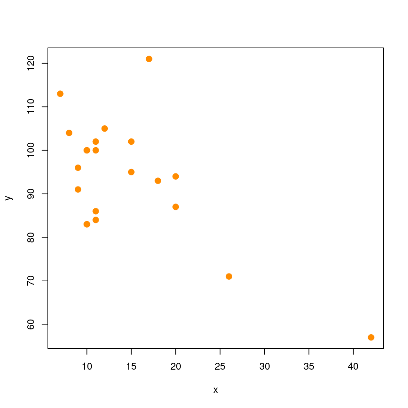

27이하로 normal하게 분포되어있는 데이터

회귀모형 적합: $y=\beta_0+ \beta_1x + \epsilon$

######## 회귀적합
model_reg <- lm(y~x, dt)
summary(model_reg)


Call:
lm(formula = y ~ x, data = dt)

Residuals:
    Min      1Q  Median      3Q     Max 
-15.604  -8.731   1.396   4.523  30.285 

Coefficients:
            Estimate Std. Error t value Pr(>|t|)    
(Intercept) 109.8738     5.0678  21.681 7.31e-15 ***
x            -1.1270     0.3102  -3.633  0.00177 ** 
---
Signif. codes:  0 ‘***’ 0.001 ‘**’ 0.01 ‘*’ 0.05 ‘.’ 0.1 ‘ ’ 1

Residual standard error: 11.02 on 19 degrees of freedom
Multiple R-squared:   0.41, Adjusted R-squared:  0.3789 
F-statistic:  13.2 on 1 and 19 DF,  p-value: 0.001769

plot(y~x, dt,pch = 20,cex = 2,col = "darkorange")
abline(model_reg, col='steelblue', lwd=2)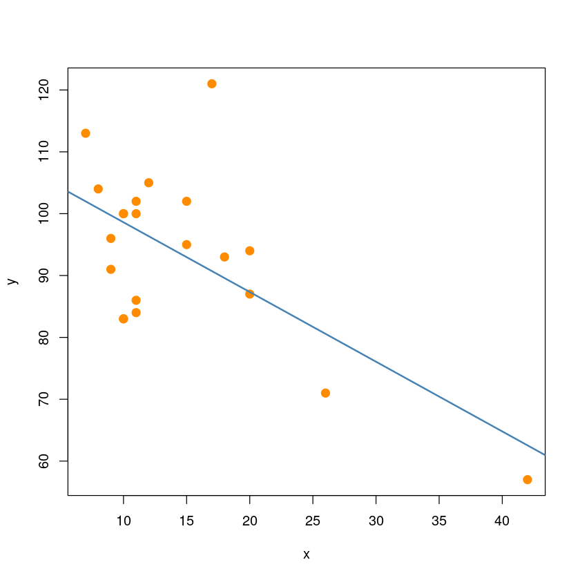

Hat Matrix

X = cbind(rep(1, nrow(dt)), dt$x)
H = X %*% solve(t(X) %*% X) %*% t(X)
diag(H)

0.0479224794510218
0.154513234296056
0.0628157755825353
0.0705452077520549
0.0479224794510218
0.0726189578463162
0.0579895935449815
0.0566699343940879
0.0798582309026469
0.0726189578463162
0.0907548450343112
0.0705452077520549
0.0628157755825353
0.0566699343940879
0.0566699343940879
0.0628157755825353
0.0521076841867129
0.65160998416409
0.0530502978659226
0.0566699343940879
0.0628157755825353

21x21행렬
0.0628157755825353 18번쨰가 큰값을 가지고 있음. leverage일 확률이 크다.

sum(diag(H))

$\sum h_{ii} = p+1 = 2$

hatvalues(model_reg)

1: 0.0479224794510218
2: 0.154513234296056
3: 0.0628157755825353
4: 0.0705452077520549
5: 0.0479224794510218
6: 0.0726189578463163
7: 0.0579895935449815
8: 0.0566699343940879
9: 0.0798582309026469
10: 0.0726189578463163
11: 0.0907548450343111
12: 0.0705452077520549
13: 0.0628157755825353
14: 0.0566699343940879
15: 0.0566699343940879
16: 0.0628157755825353
17: 0.0521076841867129
18: 0.65160998416409
19: 0.0530502978659226
20: 0.0566699343940879
21: 0.0628157755825353

hatvalues는 $h_{ii}$값 바로 나오게 하는 함수

which.max(hatvalues(model_reg))  # 가장 큰 값의 번호
hatvalues(model_reg)[which.max(hatvalues(model_reg))] ##h_{18,18}값

18: 18

18: 0.65160998416409

2*(1+1)/nrow(dt)

0.19047619047619

$h_{18,18} > 2 \bar h=2 \dfrac{p+1}{n}=2\dfrac{2}{21}=0.19047619047619$이므로 18번째 관측값이 leverage point 로 고려 가능

hatvalues(model_reg)>0.19047619047619

1: FALSE
2: FALSE
3: FALSE
4: FALSE
5: FALSE
6: FALSE
7: FALSE
8: FALSE
9: FALSE
10: FALSE
11: FALSE
12: FALSE
13: FALSE
14: FALSE
15: FALSE
16: FALSE
17: FALSE
18: TRUE
19: FALSE
20: FALSE
21: FALSE

0.19047619047619보다 큰값이 있다면 leverage point

plot(y~x, dt,pch = 20,cex = 2,col = "darkorange")
text(dt[18,],"18", pos=2)
abline(model_reg, col='steelblue', lwd=2)

이상치

잔차: $e_i = y_i - \hat y_i$

residual <- model_reg$residuals
head(residual)

1: 2.03099313777248
2: -9.57212879873313
3: -15.6039514365432
4: -8.73094035140638
5: 9.03099313777241
6: -0.334062287911925

hist(residual)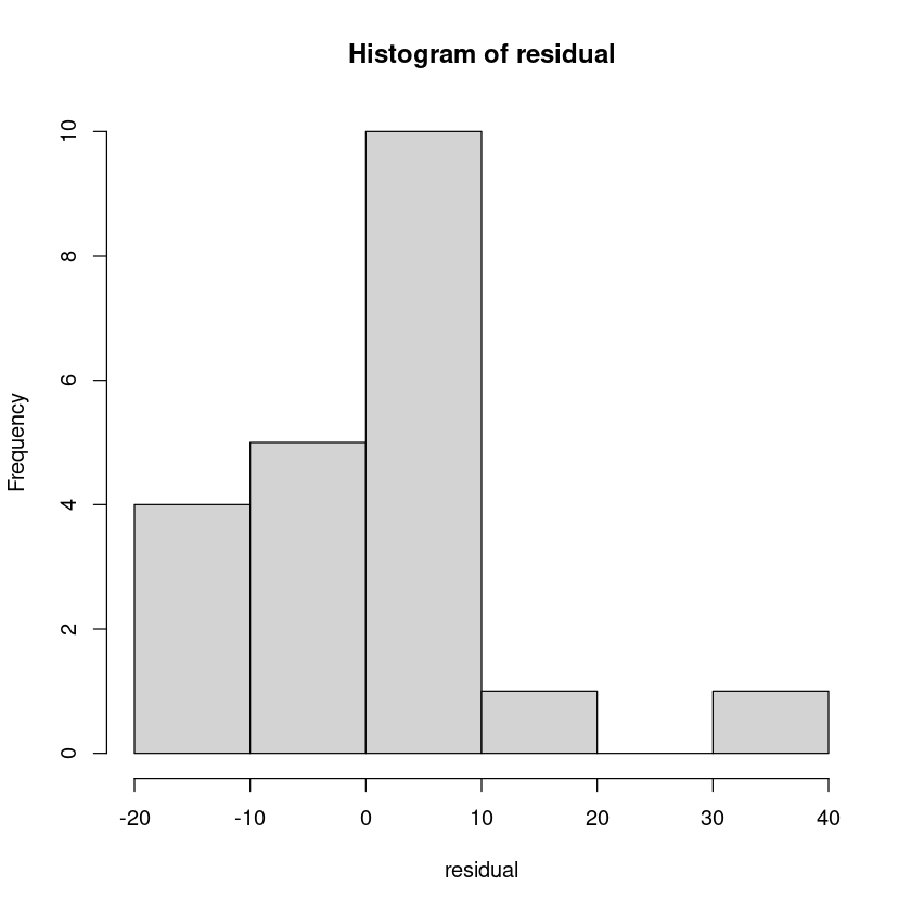

1개의 관측값이 30~40 사이에 있다. 혼자 동떨어져있는 값

내적으로 표준화된 잔차 ((internally) standardized residual)

\[r_i = \dfrac{e_i}{\hat \sigma \sqrt{1-h_{ii}}}\]: 아마도$N(0,1)$을 따를거야. 하지만 $\hat \sigma$이므로 완벽한 정규분포는 아니고 그렇다면 t분포냐? 독립이 아니므로 t분포가 아니다. N이 충분히 크다면 대략적으로 정규분포를 따른다고 볼 수 있다.

$e_i$ ~ $N(0,\sigma^2(1-h_{ii}))$

$|r_i| \geq 2$ OR $|r_i| \geq 3$이면 이상치

s_residual <- rstandard(model_reg)
head(s_residual)

1: 0.188832217420025
2: -0.944406394989665
3: -1.46226436944709
4: -0.821581550713305
5: 0.839659390272954
6: -0.0314703908632008

# 또는
s_xx <- sum((dt$x-mean(dt$x))^2) #S_xx
h_ii <- 1/21 + (dt$x- mean(dt$x))^2/s_xx #hatvalues로 구해도 됨. 혹은 X(X^TX)-1X^T로 해도 됨
### h_ii <- hatvalues(model_reg)
### h_ii <- influence(model_reg)$hat
hat_sigma <- summary(model_reg)$sigma #hat sigma
s_residual <- resid(model_reg)/(hat_sigma*sqrt(1-h_ii)) ## 내적

$h_{ii}=\dfrac{1}{n}+\dfrac{(x_i-\bar x)^2}{S_{xx}}$

hist(s_residual)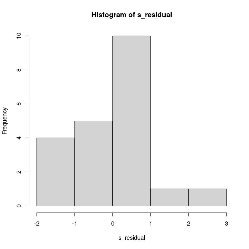

똑같은 모양인데 scaleing시켜서 0근처에서 움직이도록. 2나 3보다 크면 이상치라고 했으니 맨오른쪽에 있는 관측값이 이상치일 듯. 근데 약간 몰려있어서 애매해.

외적으로 표준화된 잔차 ((externally) standardized residual)

\[r_i^* = \dfrac{e_i}{\hat \sigma_i \sqrt{1-h_{ii}}}\]: $t(n-p-2)=(n-1-p-1)$

$\hat \sigma_i : i$번째 측정값 $y_i$를 제외하고 얻어진 $\hat \sigma$

$\hat \sigma_i^2 = \left[ (n-p-1) \hat \sigma^2 - \dfrac{e_i^2}{1-h_{ii}} \right] / (n-p-2)$

$|r_i^*| \geq t_{\alpha/2}(n-p-2)$이면 이상치

s_residual_i <- rstudent(model_reg)
head(s_residual_i)

1: 0.183968493379394
2: -0.941583351378201
3: -1.51081192291799
4: -0.814263363159438
5: 0.832862917520795
6: -0.030631827537088

# 또는
hat_sigma_i <- sqrt(((21-1-1)*hat_sigma^2 - residual^2/(1-h_ii) )/(21-1-2))
## hat_sigma_i <- influence(model_reg)$sigma
s_residual_i <- residual/(hat_sigma_i*sqrt(1-h_ii)) ## 외적

hist(s_residual_i)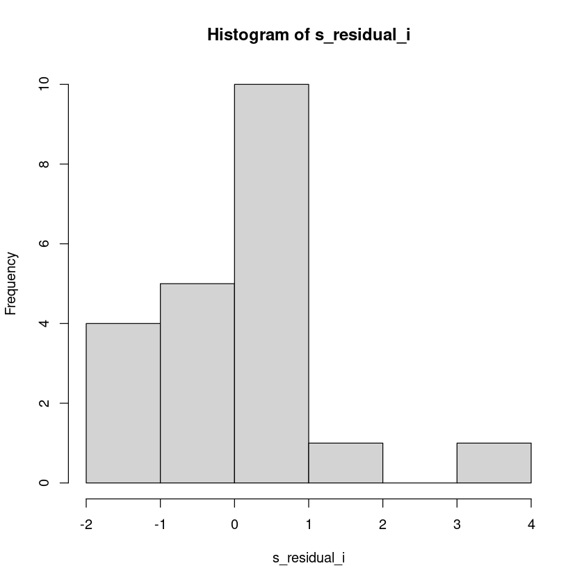

둥 떨어져있는 맨 오른쪽 관측값

which.max(s_residual_i)
s_residual_i[which.max(s_residual_i)]

19: 19

19: 3.60697972130439

qt(0.975, 21-1-2)

2.10092204024104

$t_{0.025}(21-1-1) : \alpha=5\%$

$|r_i^*| \geq t_{\alpha/2}(n-p-2)$이면, 유의수준 $\alpha$에서, $i$번째 관측값이 이상점이라고 할 수 있다.

따라서 19번째 관측값은 유의수준 0.05에서 이상점이라고 할 수 있다.

plot(y~x, dt,pch = 20,cex = 2,col = "darkorange")
text(dt[19,],"19", pos=2)
abline(model_reg, col='steelblue', lwd=2)

s_residual_i[which(abs(s_residual_i)>qt(0.975,21-2))]

19: 3.60697972130439

## 잔차그림
par(mfrow = c(2, 2))
plot(fitted(model_reg), residual,
 pch=20,cex = 2,col = "darkorange",
 xlab = "Fitted", ylab = "Residuals",
 main = "residual plot")
abline(h=0, lty=2)
plot(fitted(model_reg), s_residual,
 pch=20,cex = 2,col = "darkorange",
 xlab = "Fitted", ylab = "S_Residuals",
 ylim=c(min(-3, min(s_residual)),
 max(3,max(s_residual))),
 main = "standardized residual plot")
abline(h=c(-2,0,2), lty=2)
plot(fitted(model_reg), s_residual_i,
 pch=20,cex = 2,col = "darkorange",
 xlab = "Fitted", ylab = "S_Residuals_(i)",
 ylim=c(min(-3, min(s_residual_i)),
 max(3,max(s_residual_i))),
 main = "studentized residual plot")
abline(h=c(-3,-2,0,2,3), lty=2)
plot(fitted(model_reg), s_residual_i,
 pch=20,cex = 2,col = "darkorange",
 xlab = "Fitted", ylab = "S_Residuals_(i)",
 ylim=c(min(-3, min(s_residual_i)),
 max(3,max(s_residual_i))),
 main = "studentized residual plot")
abline(h=c(-qt(0.975,21-2),0,qt(0.975,21-2)), lty=2)
text (fitted(model_reg)[which(abs(s_residual_i)>qt(0.975,21-2))],
 s_residual_i[which(abs(s_residual_i)>qt(0.975,21-2))],
 which(abs(s_residual_i)>qt(0.975,21-2)),adj = c(0,1))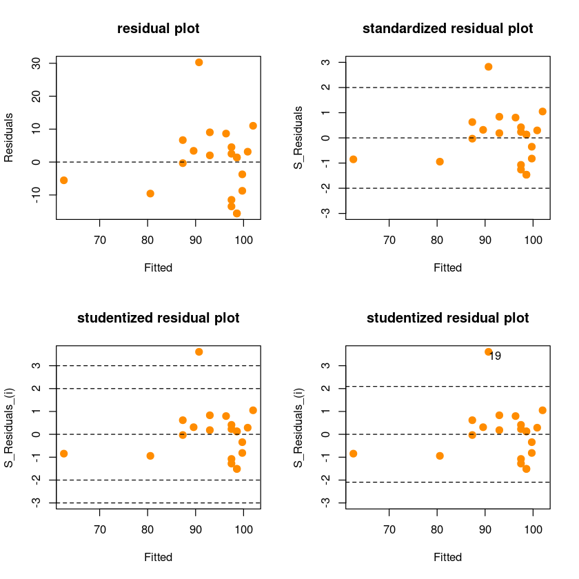

맨오른쪽 아래 그림은 $t_i^*$의 그림이고 점선은 위에는 $t_{0.025}(21-2)$, 아래는 $-t_{0.025}(19)$

정규성 검정

## 정규성 검정
par(mfrow=c(1,2))
hist(resid(model_reg),
 xlab = "Residuals",
 main = "Histogram of Residuals",
 col = "darkorange",
 border = "dodgerblue",
 breaks = 20)
qqnorm(resid(model_reg),
 main = "Normal Q-Q Plot",
 col = "darkgrey",
 pch=16)
qqline(resid(model_reg), col = "dodgerblue", lwd = 2)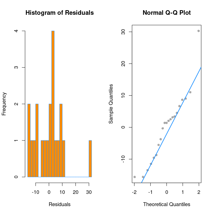

Q-Q plot에서 꼬리가 하나가 길게 나옴->이상치

## Shapiro-Wilk Test
## H0 : normal distribution vs. H1 : not H0
shapiro.test(resid(model_reg))


    Shapiro-Wilk normality test

data:  resid(model_reg)
W = 0.92578, p-value = 0.1133

기각할 수 없다. 정규분포이다.

## 독립성 검정
lmtest::dwtest(model_reg)


    Durbin-Watson test

data:  model_reg
DW = 2.0844, p-value = 0.5716
alternative hypothesis: true autocorrelation is greater than 0

### 등분산성
## H0 : 등분산 vs. H1 : 이분산 (Heteroscedasticity)
bptest(model_reg)


    studentized Breusch-Pagan test

data:  model_reg
BP = 0.0014282, df = 1, p-value = 0.9699

영향점

plot(y~x, dt,pch = 20,cex = 2,col = "darkorange")
abline(model_reg, col='steelblue', lwd=2)

influence(model_reg)

$hat

1: 0.0479224794510218
2: 0.154513234296056
3: 0.0628157755825353
4: 0.0705452077520549
5: 0.0479224794510218
6: 0.0726189578463163
7: 0.0579895935449815
8: 0.0566699343940879
9: 0.0798582309026469
10: 0.0726189578463163
11: 0.0907548450343111
12: 0.0705452077520549
13: 0.0628157755825353
14: 0.0566699343940879
15: 0.0566699343940879
16: 0.0628157755825353
17: 0.0521076841867129
18: 0.65160998416409
19: 0.0530502978659226
20: 0.0566699343940879
21: 0.0628157755825353

$coefficients

A matrix: 21 × 2 of type dbl
	(Intercept)	x
1	0.086545033	0.001045618
2	0.958749611	-0.104156236
3	-1.623423657	0.057755211
4	-1.022877601	0.040022565
5	0.384830249	0.004649436
6	0.005894578	-0.001602673
7	0.023216186	0.010379001
8	0.230329653	-0.007159985
9	0.410719785	-0.017252806
10	-0.117621441	0.031980023
11	1.595051450	-0.070799821
12	-0.437100147	0.017102603
13	-1.623423657	0.057755211
14	-1.230320253	0.038245507
15	0.412910892	-0.012835671
16	0.145243868	-0.005167222
17	0.681955144	-0.017203712
18	4.243970455	-0.347768136
19	0.569162106	0.066321856
20	-1.047739014	0.032569820
21	0.145243868	-0.005167222

$sigma

1: 11.3143301900592
2: 11.0559573770349
3: 10.6687048798294
4: 11.1219769595247
5: 11.1128596831455
6: 11.3246668862836
7: 11.2946094952564
8: 11.3083981658447
9: 11.2986143079264
10: 11.2068222590166
11: 10.9927834633216
12: 11.2881682070624
13: 10.6687048798294
14: 10.8424219439862
15: 11.2716431731807
16: 11.3198601181168
17: 11.1296641708463
18: 11.1067560007425
19: 8.62819605992093
20: 10.9771279294265
21: 11.3198601181168

$wt.res

1: 2.03099313777248
2: -9.57212879873313
3: -15.6039514365432
4: -8.73094035140638
5: 9.03099313777241
6: -0.334062287911925
7: 3.41195988236181
8: 2.52303747831988
9: 3.14207073373048
10: 6.66593771208808
11: 11.0150818188674
12: -3.73094035140638
13: -15.6039514365432
14: -13.4769625216801
15: 4.52303747831988
16: 1.39604856345675
17: 8.65002639318302
18: -5.54030616092301
19: 30.2849709674987
20: -11.4769625216801
21: 1.39604856345675

coefficients: (Intercept)=$\beta_0$, x=$\beta_1$

0.001045618 = $\hat \beta_1 - \tilde \beta_1$ : (포함하여)21개로 돌린거랑 (1번째 변수빼고)20개로 돌린거의 차이값

-0.005167222 = $\hat \beta_1 - \tilde \beta_1$ : (포함하여)21개로 돌린거랑 (21번째 변수빼고)20개로 돌린거의 차이값

값이 크면 영향점으로 생각

18번째 데이터가 살짝 커보인다.

$sigma : $\hat \sigma_{(i)}$

$wt.res : 신경쓰지말자

influence.measures(model_reg)

Influence measures of
     lm(formula = y ~ x, data = dt) :

     dfb.1_    dfb.x    dffit cov.r   cook.d    hat inf
1   0.01664  0.00328  0.04127 1.166 8.97e-04 0.0479    
2   0.18862 -0.33480 -0.40252 1.197 8.15e-02 0.1545    
3  -0.33098  0.19239 -0.39114 0.936 7.17e-02 0.0628    
4  -0.20004  0.12788 -0.22433 1.115 2.56e-02 0.0705    
5   0.07532  0.01487  0.18686 1.085 1.77e-02 0.0479    
6   0.00113 -0.00503 -0.00857 1.201 3.88e-05 0.0726    
7   0.00447  0.03266  0.07722 1.170 3.13e-03 0.0580    
8   0.04430 -0.02250  0.05630 1.174 1.67e-03 0.0567    
9   0.07907 -0.05427  0.08541 1.200 3.83e-03 0.0799    
10 -0.02283  0.10141  0.17284 1.152 1.54e-02 0.0726    
11  0.31560 -0.22889  0.33200 1.088 5.48e-02 0.0908    
12 -0.08422  0.05384 -0.09445 1.183 4.68e-03 0.0705    
13 -0.33098  0.19239 -0.39114 0.936 7.17e-02 0.0628    
14 -0.24681  0.12536 -0.31367 0.992 4.76e-02 0.0567    
15  0.07968 -0.04047  0.10126 1.159 5.36e-03 0.0567    
16  0.02791 -0.01622  0.03298 1.187 5.74e-04 0.0628    
17  0.13328 -0.05493  0.18717 1.096 1.79e-02 0.0521    
18  0.83112 -1.11275 -1.15578 2.959 6.78e-01 0.6516   *
19  0.14348  0.27317  0.85374 0.396 2.23e-01 0.0531   *
20 -0.20761  0.10544 -0.26385 1.043 3.45e-02 0.0567    
21  0.02791 -0.01622  0.03298 1.187 5.74e-04 0.0628

dfb.1_ , dfb.x : $(\hat \beta_1 - \tilde \beta_{1(i)})/$뭘로나누자
inf : 영향점인 것 같으면 *로 표시

DFFITS

DFFITS: $DFFITS(i) = \dfrac{\hat y_i - \tilde y_i(i)}{\hat \sigma_{(i)} \sqrt{h_{ii}}}$
$|DFFITS(i)| \geq 2 \sqrt{\dfrac{p+1}{n-p-1}}$이면 영향점

dffits(model_reg)

1: 0.0412740357514056
2: -0.402520687302525
3: -0.391140045474215
4: -0.224328533660804
5: 0.186855983882421
6: -0.00857173640678122
7: 0.0772239528389379
8: 0.0563034865220476
9: 0.085407472693718
10: 0.172840518129759
11: 0.331996853994253
12: -0.0944496430423618
13: -0.391140045474215
14: -0.313673908094842
15: 0.101264129345836
16: 0.0329813827461469
17: 0.187166128054405
18: -1.15577873097521
19: 0.853737107130766
20: -0.263846244162542
21: 0.0329813827461469

which(abs(dffits(model_reg)) > 2*sqrt(2/(21-2)))

18: 18
19: 19

Cook’s Distance

Cook’s Distance
$D(i) = \dfrac{\sum_{i=1}^n (\hat y_j - \hat y_j(i))^2}{(p+1)\hat \sigma^2}=\dfrac{(\hat \beta - \hat \beta(i))^T X^T X (\hat \beta - \hat \beta(i))}{(p+1) \hat \sigma^2}$
$\hat \beta(i): i$번째 관측치를 제외하고 $n-1$개의 관측값에서 구한 $\hat \beta$의 최소제곱추저량

cooks.distance(model_reg)

1: 0.000897406392870691
2: 0.0814979551507635
3: 0.0716581442213833
4: 0.0256159582452641
5: 0.0177436626335013
6: 3.87762740910137e-05
7: 0.0031305748029949
8: 0.00166820857813469
9: 0.00383194880672965
10: 0.0154395158127621
11: 0.0548101351203612
12: 0.00467762256482442
13: 0.0716581442213833
14: 0.0475978118328145
15: 0.00536121617564154
16: 0.000573584529113046
17: 0.017856495213809
18: 0.678112028575845
19: 0.223288273631179
20: 0.0345188940892692
21: 0.000573584529113046

$D(i) \geq F_{0.5}(p+1, n-p-1)$이면 영향점으로 의심

qf(0.5,2,21-2)

0.719060569091733

which(cooks.distance(model_reg) >qf(0.5,2,21-2))

없다!

COVRATIO

COVRATIO

$COVRATIO(i) = \dfrac{1}{\left[1+\dfrac{(r_i^*)^2-1}{n-p-1}\right]^{p+1}(1-h_{ii})}$

$|COVRATIO(i)-1| \geq 3(p+1)/n$이면 $i$번째 관측치를 영향을 크게 주는 측정값으로 볼 수 있음

covratio(model_reg)

1: 1.16589181683219
2: 1.19699897676296
3: 0.936347397341839
4: 1.11510268993929
5: 1.08504108257728
6: 1.20131998275497
7: 1.17015757898673
8: 1.17423726760803
9: 1.19966823450598
10: 1.15209128858604
11: 1.08783960928084
12: 1.18326164825873
13: 0.936347397341839
14: 0.992331347870996
15: 1.15904532932769
16: 1.18673688685713
17: 1.09643883044992
18: 2.95868271380702
19: 0.396431612340971
20: 1.04257281407241
21: 1.18673688685713

which(abs(covratio(model_reg)-1) > 3*(1+1)/21)

18: 18
19: 19

영향점

summary(influence.measures(model_reg))

Potentially influential observations of
     lm(formula = y ~ x, data = dt) :

   dfb.1_ dfb.x   dffit   cov.r   cook.d hat    
18  0.83  -1.11_* -1.16_*  2.96_*  0.68   0.65_*
19  0.14   0.27    0.85    0.40_*  0.22   0.05

*였떤 점만 뽑아서 보여줘ㅡ

## 18제거 전후
plot(y~x, dt,pch = 20,
 cex = 2,col = "darkorange",
 main = "18번 제거")
abline(model_reg, col='steelblue', lwd=2)
abline(lm(y~x, dt[-18,]), col='red', lwd=2)
text(dt[18,], pos=2, "18")
legend('topright', legend=c("full", "del(18)"),
 col=c('steelblue', 'red'), lty=1, lwd=2)
# high leverage and high influence, not outlier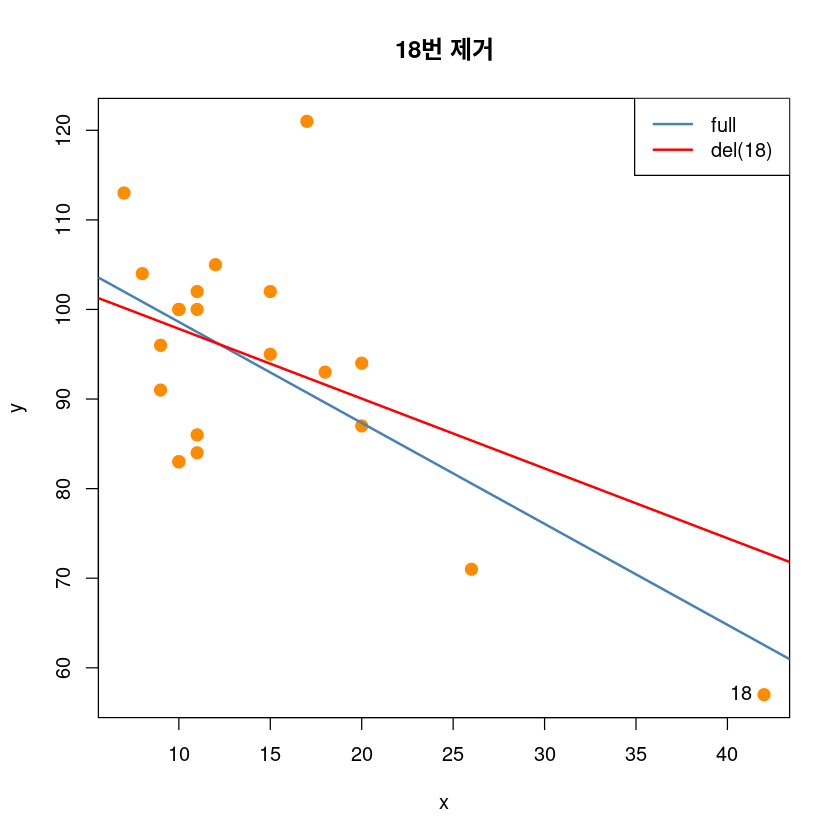

## 19제거 전후
plot(y~x, dt,pch = 20,
 cex = 2,col = "darkorange",
 main = "19번 제거")
abline(model_reg, col='steelblue', lwd=2)
abline(lm(y~x, dt[-19,]), col='red', lwd=2)
text(dt[19,], pos=2, "19")
legend('topright', legend=c("full", "del(19)"),
 col=c('steelblue', 'red'), lty=1, lwd=2)
# not leverage and high influence, outlier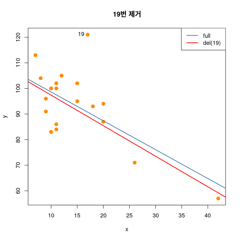

19번째는 살짝 애매하다.

## 18, 19제거 전후
plot(y~x, dt,pch = 20,
 cex = 2,col = "darkorange",
 main = "18,19번 제거")
abline(model_reg, col='steelblue', lwd=2)
abline(lm(y~x, dt[-c(18,19),]), col='red', lwd=2)
text(dt[c(18,19),], pos=2, c("18","19"))
legend('topright', legend=c("full", "del(18,19)"),
 col=c('steelblue', 'red'), lty=1, lwd=2)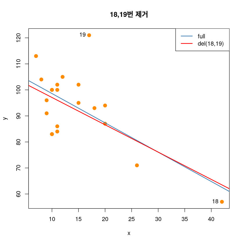

회귀진단 그림

## 회귀진단 그림
par(mfrow = c(2, 2))
plot(model_reg, pch=16)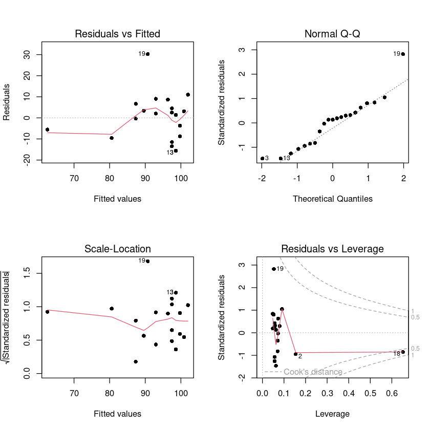

왼쪽위에: $e_i, \hat y_i$그림
왼쪽아래: $\sqrt{|r_i|}$
오른쪽 아래: 이상치, 영향점, leverage다볼수잇당

06. 회귀진단 실습